
Section 2.8 Parametric Surfaces
- Examples:
See the list of example Parametric Surfaces on the Examples submenu of the CalcPlot3D main menu. See more about the Examples menu in Section 4.6.
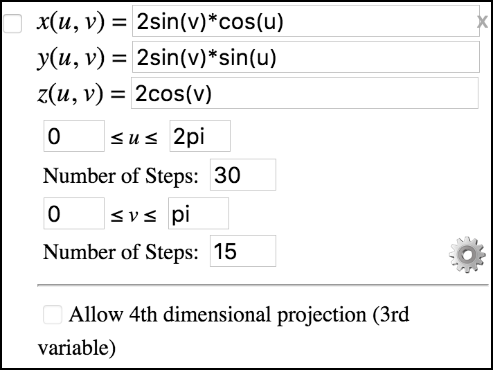
To add a parametric surface to the plot, select the option Parametric Surface on the Add to graph drop-down menu. You'll see an object dialog appear like the following:
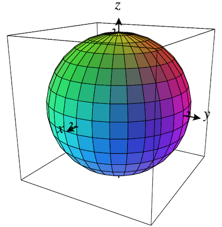
Now let's plot the default parametric surface.

Clear the plot by clicking the clear plot button.
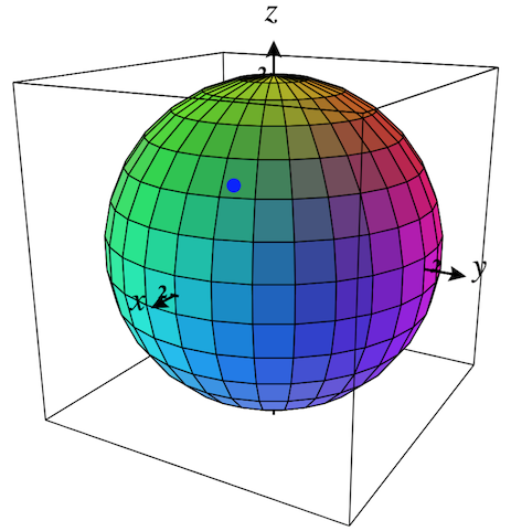
Then check the checkbox in the upper-left corner of this object to plot the default parametric surface. It should look like Figure 2.8.2.
You can vary the ranges and the number of steps for both \(u\) and \(v\) to control the rectangular region of the \(uv\)-plane used to generate the parametric surface.
Use the settings button ⚙ to adjust surface settings. For a discussion of the options, see Section 2.11.
The last option is not yet implemented. It is intended to allow 4th dimensional parametric surfaces to be visualized, but it has not yet been worked out.
\(\Large\textbf{Tracing a Parametric Surface on the 2D Traceplot:}\)
When a parametric surface is the primary surface object in CalcPlot3D's 3D plot, the 2D Trace Plane will use the variables \(u\) and \(v\) to allow you to see the effect of varying these parameters on the location of the associated point on the parametric surface.
To see this feature, open the 2D Trace Plane using the toolbar button.

The traceplane should appear like Figure 2.8.3.
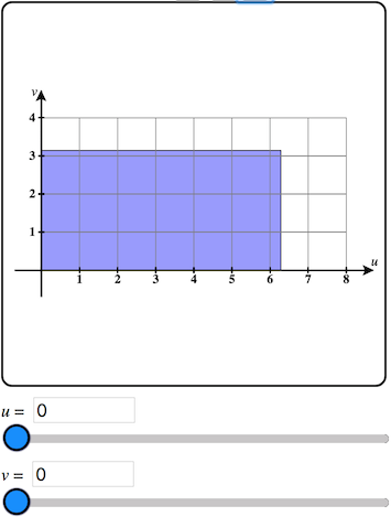
Now click on the trace plane and an input point will appear on the trace plane where you click and the corresponding trace point should appear on the parametric surface. The corresponding values of \(u\) and \(v\) are displayed in the textbox/sliders below the \(uv\)-plane.
These sliders can be very helpful to show how varying each of these parameters corresponds to the points obtained on the parametric surface.
See Figure 2.8.4 and Figure 2.8.5.
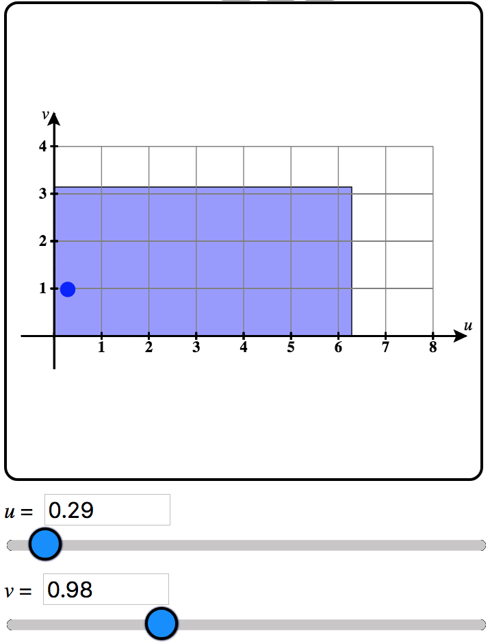
You can also see the coordinates of the corresponding trace point on the parametric surface in the green message line above the 3D plot.

\(\Large\textbf{Adjusting the}\,uv \Large\textbf{-domain of a Parametric Surface on the 2D Traceplot:}\)
You can even directly adjust the rectangular region in the \(uv\)-plane that defines the parametric surface. To do this, click and drag on any of the four edges of this recrtangular region. You should be able to adjust each edge and observe how this affects the corresponding parametric surface.
Note that while adjusting these edges, they will lock onto multiples and fractions of \(\pi\text{,}\) as many parametric surfaces use radians.