
Section 2.10 Parameter Sliders
Parameters can be used in surfaces, curves or vector fields to show the effect of varying these parameters on the plot.
They are useful for exploration, for demonstration of relationships, and for animation.
Currently, possible parameters are a, b, c, d, and t. More parameters may be added in the future. And note that t cannot be used as a parameter in Space Curves, since it is already being used in this context as the independent variable.
When you use a parameter in a surface, curve or vector field, a corresponding slider object will be added automatically when you graph the object.
The parameter \(t\) will also be automatically added to the plot when you add a vector field. See more about this feature in the chapter on differential equations in Subsection 6.2.1.
Subsection 2.10.1 Working with Parameter Sliders
Although the corresponding parameter slider will automatically be added to the plot when you use a new parameter in another object, you may wish to create and configure one first. To do this, select the option slider on the Add to graph drop-down menu. You'll see an object dialog appear like the following:
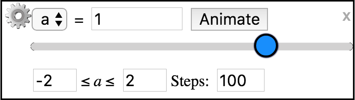
By default, the new slider will be assigned the next available parameter name, although you can then use the drop-down menu to select which parameter you wish the slider to represent. It is even possible for you to have more than one slider for a given parameter, perhaps with different ranges or number of steps.
Each slider has a textbox that allows you to enter an initial value for the parameter. Entering a value here will automatically affect any object in the plot that uses this parameter in its definition.
The range of values for this parameter is given along the bottom of the slider dialog. You can specify this range by adjusting these values. This will affect the values obtained in the textbox when using the slider and will affect what values are used in animation of this parameter.
The number of steps can also be adjusted for each parameter. If you wish to used just integer steps in your animation or slider, you will need to consider the difference between the max and min range values and then use this natural number as your number of steps.
Clicking the Animate button on a slider will cause the value of this parameter to automatically vary, starting with the minimum value and progressing through the number of steps specified to reach the maximum range value. To speed up this animation, use a smaller number of steps. To slow it down, use a larger number of steps.
When animation of a parameter starts, the label on the Animate button changes to read Pause. When you click it again, it will continue with the animation.
Subsection 2.10.2 Parameter Settings, ⚙
If you click on the settings button ⚙ on a slider object, you will see the following menu.
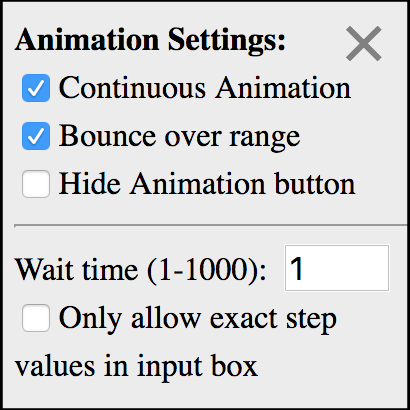
The options are:
- Continuous Animation:
(the default) Causes animation to continue once it has passed through the range of slider values.
- Bounce over range:
(the default) If Continuous Animation is selected, this option causes animation to continue by going back in reverse through the range of slider values. Once it reaches the minimum value again, it will reverse again and go back through the values in the forward direction, etc.
- Hide Animation button:
Causes the Animate button to be hidden. This is most useful when creating dynamic figures. For more information on creating dynamic figures see Appendix B.
- Wait time (1-1000):
This option gives you another way to control the speed of the animation (in addition to using more steps for slower animation).
- Only allow exact step values in input:
If this option is selected, only values that would come up using the slider's exact steps will be allowed in the textbox. If it is unselected, other values are allowed.
Subsection 2.10.3 Ways to Use Parameters
-
To show function transformations:
Example: Enter
z = c(x-a)^2 + d(y-b)^2 + tVarying the various parameters will then show how the paraboloid is transformed.
- a
shifts paraboloid \(a\) units in the positive \(x\)-direction
- b
shifts paraboloid \(b\) units in the positive \(y\)-direction
- t
shifts paraboloid \(t\) units in the positive \(z\)-direction
- c
scales the \(x\)-components of the paraboloid by a factor of \(c\) in the vertical \(z\)-direction
- d
scales the \(y\)-components of the paraboloid by a factor of \(d\) in the vertical \(z\)-direction
-
To show various curves in a family:
Example: Hypocycloids and Epicycloids
Clear the plot.
Add a space curve to the plot by selecting Add a space curve from the Add to graph dropdown menu.
Zoom out to -8 to 8 in both \(x\)- and \(y\)-directions using the Zoom-out button.
Now enter the following parametric function:
x = a cos(t) - cos(at),y = a sin(t) - sin(at),z = 0.Enter a range of 0 to 2pi for \(t\text{,}\) and select Restrict view to 2D on the space curve dialog.
-
A parameter slider object should have automatically appeared for the parameter
a. Vary the value ofausing the slider or enter values of 2, 3, or -4.Notice that when the value of
ais a positive integer, you will see an epicycloid withacycles (petals).When the value of
ais a negative integer, you will see a hypocycloid withacycles (points). Now it would be nicest if we only showed these integer values for the parameter
aas the slider is moved. To do this, click on the parameter dialog so it displays all its options. Set the values ofato range from -10 to 10 and then enter 20 steps. This will force the parameterato only take on the integer values between -10 and 10, inclusive. Now try the slider again to see the series of epicycloids and hypocycloids displayed one after another.
To show solution curves for a system of DEs: This is really a special case of the previous category, but it is a distinct application. See an example in Subsection 6.2.1 on exploring systems of differential equations using CalcPlot3D.
To show level surfaces: You can add an Implicit Surface to the plot and enter the level surface equation of \(f(x, y, z) = c\) using parameter \(c\text{.}\) Then you can vary the parameter to view the various level surfaces of this function of three variables. See more about this example in the second part of Section 5.6, titled Method 2.
-
To create animations:
Click on the following link to open CalcPlot3D with an example of how parameters can be used for animation.
Cycloid animation exploration in CalcPlot3D app
In the first displayed example, you will see three object dialogs on the left side of the screen. (See Figure 2.10.2 below.)
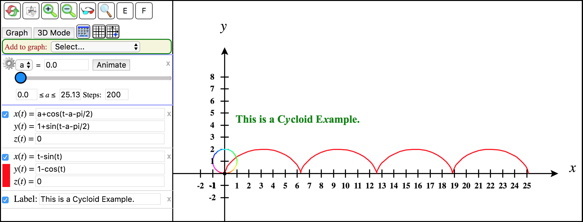
Figure 2.10.2. Cycloid animation objects The bottom object is the Label object stating that “This is a Cycloid Example.”
The middle object is the red cycloid curve in parametric form.
Finally, the first object is the one we will animate using the parameter
a. It is a circle that is animated to show it rolling along the \(x\)-axis to trace out the cycloid curve. To make it look more like it is rolling, we have left the color to vary in hue as it would for a 3D space curve. We also forced the point to appear on the circle (that traces out the cycloid) by entering a trace value of \(t = 0\) and selecting the Trace checkbox on this space curve object. Click on this dialog to see this.To animate this circle to roll along the \(x\)-axis and trace out the cycloid curve, click the Animate button on the
aparameter slider.Note that this example also shows an example of a script with three steps. You can view the various steps using the exploration dialog that should have appeared in the upper right corner of the app window. See Figure 2.10.3.
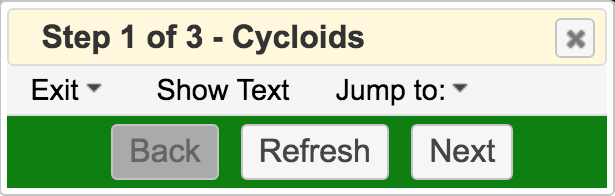
Figure 2.10.3. Exploration dialog for Cycloid exploration To view the second animation example, click the Next button on the exploration dialog.

Figure 2.10.4. Epicycloid animation This example will animate tracing out an epicycloid as a circle rolls around the outside of a circle.
Try it out by clicking on the Animate button on the
aparameter slider.Note that the curves are color-coded with the green curve being the circle on which the epicycloid is created, the blue curve is the epicycloid itself, and the black curve is the circle being animated to roll around the green circle tracing out the epicycloid. Again the trace point is displayed so you can see it, showing how it traces out the epicycloid curve as the small black circle rolls around the green circle.
Clicking the Next button again will display the third example, showing how a hypocycloid is traced out as a small black circle rolls around the inside of a larger green circle.
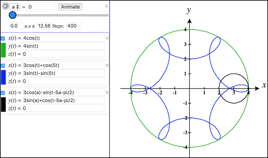
Figure 2.10.5. Hypocycloid animation