CalcPlot3D Help

Section 2.3 Vector Fields

Examples:

See the list of example Vector Fields on the Examples submenu of the CalcPlot3D main menu. See more about the Examples menu in Section 4.6.

To add a vector field to the plot, select the option Vector Field on the Add to graph drop-down menu. You'll see an object dialog appear like the following:

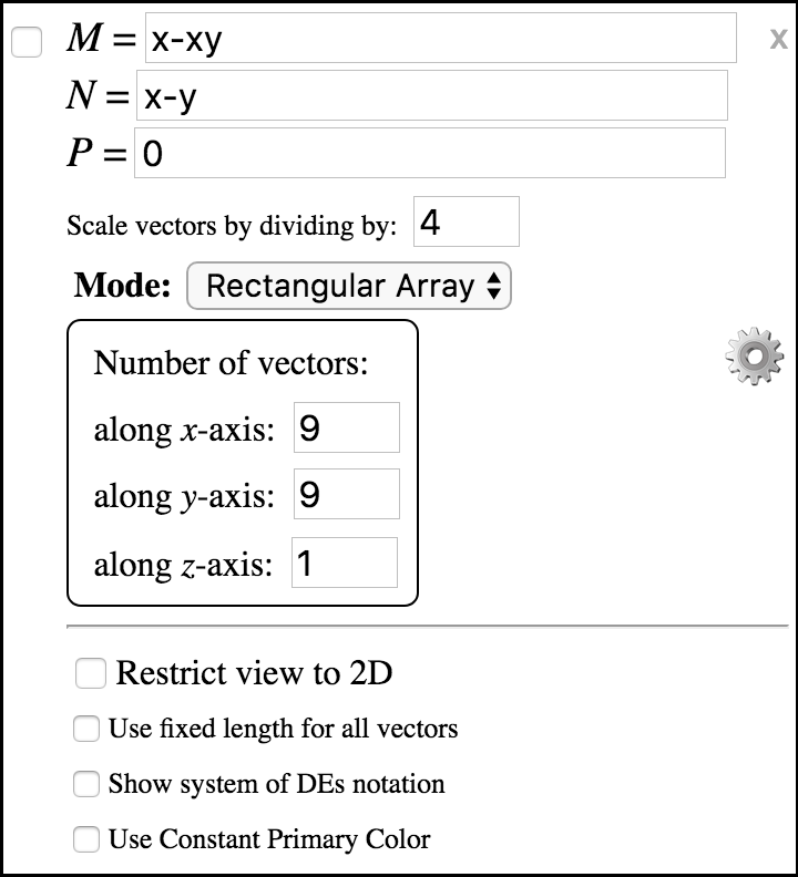
Now let's plot the default vector field.

Clear the plot by clicking the clear plot button.

Then check the checkbox in the upper-left corner of this object to plot the default vector field.

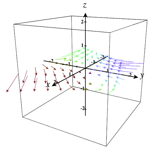
This vector field happens to be a 2D vector field, but it is plotted in a 3D plot by default. It should look like Figure 2.3.2. To quickly change the view to be above the \(xy\)-plane, select the Restrict view to 2D option. Now your view should look like Figure 2.3.3. Note that in 2D, the Use Constant Primary Color option is selected by default. When this option is not selected, the vectors are colored based on their three components similarly to the way faces of a surface are colored based on the three components of their normal vectors.

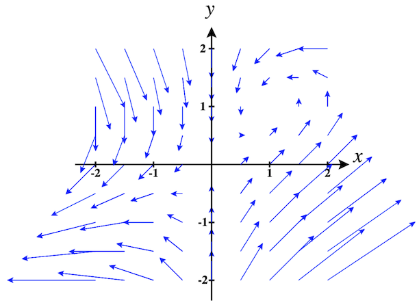
This vector field is still fairly easy to read, but sometimes the vectors may be very difficult to read because of how they overlap.

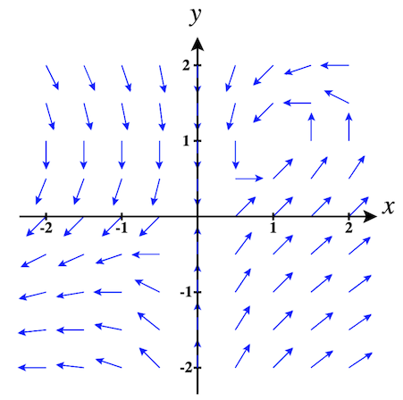
There are a couple options for dealing with this. One option is to force all vectors in the vector field to have the same fixed length. Select the checkbox labeled Use fixed length for all vectors to see how this looks. It should appear like Figure 2.3.4.

Another way to vary the vector lengths in a vector field so that they do not overlap is to adjust the scalefactor, labeled Scale vectors by dividing by. By default, vectors in a vector field are divided by 4 to scale them down. You can adjust this value to see how it affects the plot. To see all vectors in the vector field at the natural length, change this value to 1.

The Number of vectors along each axis can be adjusted to change the appearance and refinement of the vector field. When in 2D mode, we just need to adjust the number of vectors along the \(x\)- and \(y\)-axes, and keep just one vector along the \(z\)-axis. But when in 3D mode, you'll want to change the number of levels along the \(z\)-axis to be more than one.

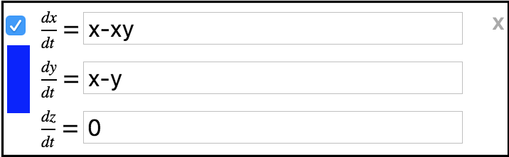
Note that if you are considering a system of differential equations, you also have the option of changing the notation of the components of the vector field to use differential notation. Select the option to Show system of DEs notation and the components of the vector field should look like those here:

\(\Large\textbf{3D Vector Fields:}\)

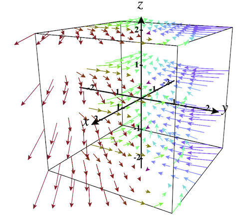
To obtain a 3D vector field, deselect the option to Restrict view to 2D and change the number of vectors along the \(z\)-axis to be more than 1. For example, if you change this value to 4 and also deselect the option to Use Constant Primary Color, the view will look like Figure 2.3.5.

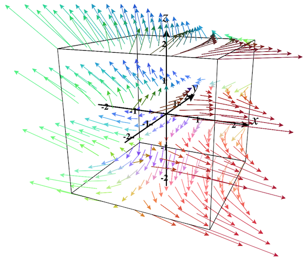
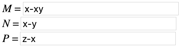
Changing the third component to be non-zero, say \(P = z - x\text{,}\) and rotating the view a little, we obtain a plot like Figure 2.3.6. The definition of the vector field is now:

Note that 3D Glasses mode would be quite helpful for 3D vector fields. Give it a try!

\(\Large\textbf{Vector Field Modes:}\)

Every vector field we've looked at so far has been in Rectangular Array mode. Now let's consider the other mode options provided here. Although these modes can be used in 2D mode, I think they are most useful when viewed in 3D.

Spherical Array:

Instead of showing vectors at a rectangular grid of points as is done in the Rectangular Array mode, Spherical Array mode places vectors at points on spheres (or circles in 2D).

Instead of specifying the number of vectors in each axis direction, Spherical Array mode uses the number of vectors on each circle (parallel to the \(xy\)-plane), the number of concentric spheres (or concentric circles in 2D), and the number of circular steps in the vertical \(z\)-direction.

Cylindrical Array:

In this mode places vectors at points on cylinders (or circles in 2D).

Cylindrical Array mode uses the number of vectors on each circle (parallel to the \(xy\)-plane), the number of concentric circles, and the number of levels in the vertical \(z\)-direction.

Note that the Settings button ⚙ in Vector Fields does not yet do anything.