
Section 5.1 Vector Explorations
Much of multivariable calculus depends, to some degree, on a clear understanding of vectors. To address the geometric nature of vectors and help students to explore the geometric significance of vectors operations, a special mode exists in CalcPlot3D titled, Vector Operations.
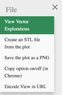
To access these Vector Explorations, open the main menu ☰ and select the View Vector Explorations option on the File menu.
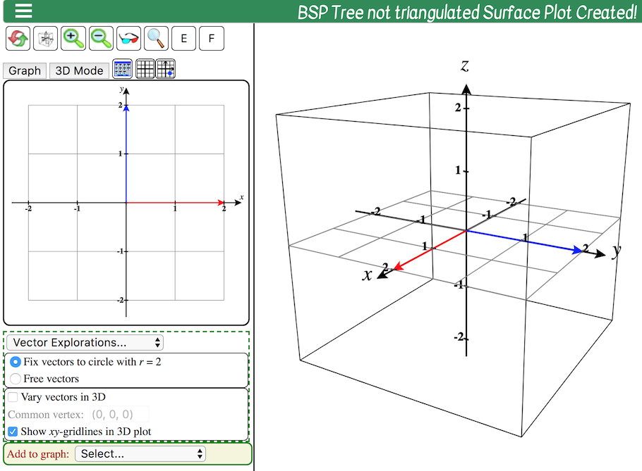
Once it is open, you should see the following view of the app, showing the 2D Trace Plot on the left and the Vector Exploration control panel just below it, with a dashed green border.
\(\Large\textbf{General Options:}\)
In each exploration, you can adjust the red and blue vectors by clicking and dragging the tip of either vector.
By default, the two vectors are fixed with a length of 2. This allows for the geometric significance of some of the vector operations to be more clear.
However, you can choose instead to free the vectors (clicking on Free vectors), so that you can adjust the lengths of each one to see the effect. Note that when you select this option, a new panel will open below allowing you to vary the components of each vector using a textbox or slider.
The Common Vertex is \((0, 0, 0)\text{,}\) by default. Eventually this vertex will be able to be changed, but not yet.
By default, there are gridlines shown in the \(xy\)-plane to help make vectors in the \(xy\)-plane more clear. Deselect the option Show \(xy\)-gridlines in 3D plot to hide these gridlines. They may be distracting when viewing the vectors in 3D.
By default, the two vectors are kept in the \(xy\)-plane, but you can explore the two vectors in 3D by selecting the option to Vary vectors in 3D, as you can see in Figure 5.1.2.
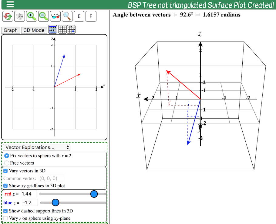
Note that the vectors in the 2D trace plot show only the projections of the red and blue vectors onto the \(xy\)-plane, while the 3D plot shows the 3D vectors. Dashed lines help to emphasize the 3D location of the tip of each vector.
Also note that several new options are provided when Vary vectors in 3D is selected.
- \(z\)-coordinate sliders
These allow you to vary the \(z\)-coordinates of the red and blue vectors.
- Show dashed support lines in 3D
Displayed by default to help visualize the 3D nature of each 3D vector.
- Vary \(z\) on sphere using \(xy\)-plane
This option allows for you to vary the vectors on the 2D trace plane forcing the vectors to have a common length in 3D. When this option is not checked, clicking and dragging either red or blue vector in the 2D trace plane only affects the \(x\)- and \(y\)-components of the vector, leaving the \(z\)-component unchanged.
Note that some additional options will be provided in some of the explorations described below. These will be described below, where available.
\(\Large\textbf{List of Vector Explorations:}\)
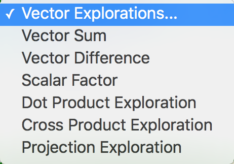
Clicking on the Vector Explorations dropdown menu allows you to select which vector operation to explore.
- default mode:
-
When the vector explorations mode is first selected (or when the dropdown option “Vector Explorations...” is selected), no particular vector operation is selected and the user can simply explore the two vectors using the various available options.
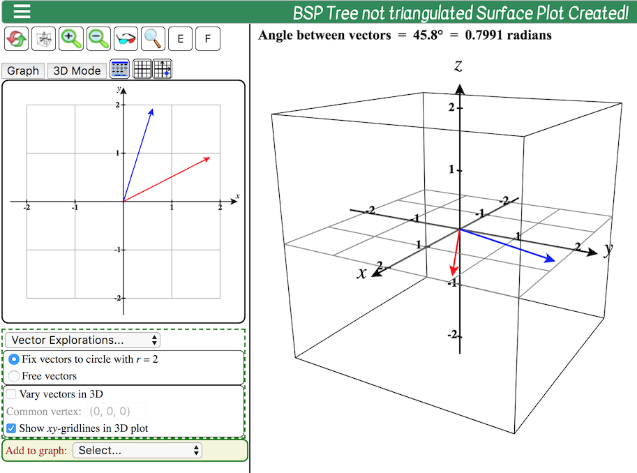
Figure 5.1.3. Exploring the angle between two vectors - Vector Sum:
-
Selecting the Vector Sum exploration displays not only the red and blue vectors, but also the resultant vector obtained by adding the blue vector to the red vector. Additionally a copy of the blue vector is placed so its tail rests at the tip of the red vector to demonstrate the tail-to-tip method of adding vectors geometrically.

Figure 5.1.4. Exploring the sum of two vectors - Vector Difference:
-
Similarly, the Vector Difference exploration displays the geometric interpretation of the differnce of two vectors. Since there are at least two ways to think of this, two options are given in this mode, allowing both to be explored visually.
Option 1 displays the most useful interpretation of a vector difference, showing its tail at the tip of the vector being subtracted and its tip at the tip of the vector coming first in the difference. That is, the vector \(\overset{\rightharpoonup}{\mathbf v} - \overset{\rightharpoonup}{\mathbf u}\) will go from the tip of vector \(\overset{\rightharpoonup}{\mathbf u}\) to the tip of vector \(\overset{\rightharpoonup}{\mathbf v}\text{.}\)

Figure 5.1.5. Exploring the difference of two vectors Option 2 displays a second interpretation of the vector difference. In this case, \(\overset{\rightharpoonup}{\mathbf v} - \overset{\rightharpoonup}{\mathbf u}\) is represented as the vector sum, \(\overset{\rightharpoonup}{\mathbf v} + (-\overset{\rightharpoonup}{\mathbf u})\text{.}\) Then the negative of vector \(\overset{\rightharpoonup}{\mathbf u}\) is added, showing its tail at the tip of the vector \(\overset{\rightharpoonup}{\mathbf v}\text{.}\)

Figure 5.1.6. Exploring the difference of two vectors - Scalar Factor:
-
This option shows the scalar product of the blue vector, here named \(\overset{\rightharpoonup}{\mathbf u}\) multiplied by the scalar, \(c\text{.}\) This exploration option provides a textbox and slider to adjust the value of the scalar, \(c\text{.}\)

Figure 5.1.7. Exploring the scalar product - Dot Product Exploration:
-
This exploration shows the value of the dot product of the red and blue vectors as well as the angle between them.

Figure 5.1.8. Exploring the dot product of two vectors - Cross Product Exploration:
-
This exploration shows a red vector in the 3D plot to represent the cross-product vector formed by taking the cross product of the red and blue vectors in an order specified by the Order option tab. The cross product's magnitude and the angle between the two vectors are displayed at the top of the 3D plot.
For this exploration, it is especially helpful select the option to Vary vectors in 3D, so that you can see how the cross product vector is affected when the vectors forming it are not both on the \(xy\)-plane.

Figure 5.1.9. Exploring the cross product of two vectors - Projection Exploration:
-
This exploration allows you to explore the projection of the blue vector onto the red vector. The projection vector is displayed in orange. Note that you also have the option here to display the \(\overset{\rightharpoonup}{\mathbf u}\)-perp vector (the vector component of the vector \(\overset{\rightharpoonup}{\mathbf u}\) that you would need to add to the projection vector to obtain \(\overset{\rightharpoonup}{\mathbf u}\)).

Figure 5.1.10. Exploring the projection of one vector onto another